Wednesday, December 19, 2012

Simple direct quadrilaterals found with the shoelace formula

The shoelace formula can computes the area of a quadrilateral  from the points coordinates . The formula requires that the points are taken clockwise or counter clockwise,  that is a quadrilateral must not be self crossing.
A criterion implemented in python was proposed to check if two segments are intersecting, which should be the case for a self-crossing quadrilateral.

With four points, there is  4!=24 ways to calculate the area. With points defining a square, according to the points order, the area takes three values: -2, 0 and 2 for indirect, self crossing and direct square:
The first point is the purple one.
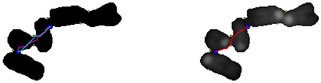
The first square (top left in red) defined by the points (1, 0), (2, 1), (1, 2), (0, 1):

((1, 0), (2, 1), (1, 2), (0, 1)) False 2.0

is detected as non self crossing (False), and the shoelace formula gives an area equal to 2 as waited  for this direct square. There is a problem for some self crossing quadrilaterals:
((1, 0), (2, 1), (0, 1), (1, 2)) False 0.0
((1, 0), (1, 2), (2, 1), (0, 1)) True 0.0

The second quadrilateral is not detected as self crossing, however the shoelace formula yield an area equal to zero, as the third quadrilateral which is correctly dtected as self crossing (True). The last quadrilateral (blue one, down right):

((0, 1), (1, 2), (2, 1), (1, 0)) False -2.0

is correctly deteted as non self crossing (False) and indirect with a negative "area" equal to -2

Trying with points yielding non convex quadrilaterals yields six values -0.95,-0.65,  -0.4, 0.4, 0.65,  0.95. None is detected as self crossing:
With other points defining a possible convex quadrilateral:
Several values are found. The maximal area value : 1.465, corresponds to the four simple quadrilaterals (non self crossing):

((1.1, 0.3), (1.7, 1.4), (1, 2), (0, 1)) False 1.465
((1.7, 1.4), (1, 2), (0, 1), (1.1, 0.3)) False 1.465
((1, 2), (0, 1), (1.1, 0.3), (1.7, 1.4)) False 1.465
((0, 1), (1.1, 0.3), (1.7, 1.4), (1, 2)) False 1.465

It seems that the maximal area value found from the set of 24 possible quadrilaterals correspond to simple direct quadrilaterals, thus testing if the four points define a non self crossing quadrilateral may not be usefull.

January 3, 2013:
The script is modified so that the quadrilaterals are plotted with matplotlib.patches.Polygon:


Download code
Play with the code on cloud.sagemath.com

Wednesday, November 7, 2012

Looking for a geodesic distance to resolve touching chromosomes

In the previous post, from a cluster of touching mouse chromosomes:
DAPI stained mouse chromosomes
points belonging to negatively curved domains of a contour can be isolated :
To separate the chromosomes, it is tempting to cut between the closest pairs of points.
Python provides itertools.combinations(); the closest pairs of points are in the set of the combinations of every pairs of points:


Each line shows the euclidian distance between two points, the four shortest lines correspond more or less to the contact domains between the chromosomes, cuting along them provides a way to separate the chromosomes.

It should be possible to do better by using a geodesic distance between the points, that is using a path inside the cluster of chromosomes. In the following example: two paths (depending on the chosen pixel neighborhood) between the two blue points were overlaid on a binary image (background is set to 255 and the foreground to 0).
the cluster contourthe cluster contour

 The path were determined as follow using skimage 0.8dev:

graph.route_through_array(negbin ,p1,p2,fully_connected=False)
 or
 graph.route_through_array(negbin ,p1,p2,fully_connected=True)

 with negbin, the negative binary image and p1, p2 the two points figured in blue.

If the background (0) is set to 255 (white) in the grey scale image:

 the path (red) between the two points can be determined by minimizing the "greyscale cost", that is through the valleys between the two points is the image is viewed as a landscape.

All the paths can be determined (blue):Those paths in blue were obtained from the previous binary image:


The paths were sorted according to their cost :


 The four paths with the smallest cost are figured in red, they are "inside" the cluster. Some paths are partially "outside" the cluster and thus are not geodesic routes inside the cluster.
Now if paths are calculated from a 8 bits greyscale image where the background was set to 255 (a naïve idea supposed to prevent a path to go "outside" a cluster):

some routes between two points, go along the contour. The two first routes to with the smallest costs do correspond to touching domains between the chromosomes. However when routes with higher cost are selected:
some correspond to the cluster contour and not to contact domains between the chromosomes, because the cost (sum of pixels grey value) along the contour is probably lower than the cost of a shorter path which have to climb over a contact domain between two chromosomes.

Additional features may distinguish routes belonging to contour from those providing solution to separate chromosomes:
red route on the right resolve touching chromosomes
Minimal cost routes are still better to separate chromosomes than routes obtained with euclidian distance:
The shortest path (on the right) cuts inside the chromosome


Download code

Friday, October 26, 2012

Trying to separate touching mouse chromosomes

In the previous post, from a cluster of touching mouse chromosomes:


points belonging to negatively curved domains of a contour can be isolated :
Yellow points belong to negatively curved domains of the contour.
To separate the chromosomes, it is tempting to cut between the closest pairs of points.

Let's make combination of pairs of points belonging to the contour:

Python provides itertools.combinations(); the closest pairs of points are in the set of the combinations of every pairs of points:

Path between two points belonging to the countour:

Each line shows the euclidian distance between two points, the four shortest lines correspond more or less to the contact domains between the chromosomes, cuting along them provides a way to separate the chromosomes.
It should be possible to do better by using a geodesic distance between the points, that is using a path inside the cluster of chromosomes. In the following example:

On the left, two paths (depending on the chosen pixel neighborhood) between the two blue points were overlaid on a binary image (background is set to 255 and the foreground to 0). The path were determined as follow using skimage 0.8dev:
graph.route_through_array(negbin ,p1,p2,fully_connected=False)
 or
 graph.route_through_array(negbin ,p1,p2,fully_connected=True)

  • negbin: the negative binary image
  • p1, p2: the two points figured in blue.

On the right the background (0) was set to 255 (white), the path (red) between the two points was determined by minimizing the "greyscale cost", that is through the valleys between the two points is the image is viewed as a greyscaled landscape.

All the paths can be determined (left), and then the paths can be sorted according to their cost (right). The four paths with the smallest cost are figured in red (left).


Download code.

or see bellow:


Wednesday, October 24, 2012

Contour : looking for negatively curved domains

A contour was previously explored with the convexity defects  algorithm implemented in opencv. Some highly curved domains  failed to be detected because of the contour shape.
Curved domains missed by convexity defects detection

Using polygonal approximation imlemented in skimage 0.8 dev, positively curved domains as well as negatively curved domains on a contour can be sorted:
Contour of a chromosomes cluster (blue), polygonal approximation (yellow). Red points: positive curvature. Yellow points: negative curvature.

From a segmented particle, a polygonal approximation of the contour is extracted.
Points of the polygon are used to compute an angle between two consecutive vectors (Here using the complex affix of vectors):

Positive angles correspond to convex domains and negative angles to concave domains.


The code has to be modified to filter angles according to a given range. 

The code can be modified as follow to filter angles corresponding to curved domains:

  • positive = table[(135>table[:,2]) & (table[:,2]>45)]
  • negative = table[(-45>table[:,2]) & (table[:,2]>-135)]
Curved domains on polygonal approximation of a chromosomes cluster contour.

Download code


Saturday, July 21, 2012

Touching chromosomes, overlapping chromosomes, single chromosomes and their convexity defects


Let's start with convexity defects (blue circles) detected in totally overlapping chromosomes:


The convexity defects can be directly used to resolve the two overlapping chromosomes, the script is used with d>1000 (see the two previous posts).
When the chromosomes partially overlap, we can have less than four points detected:

As in the previous post, touching chromosomes produce convexity defects. In the following example of two small chromosomes, the two convexity defects detected surrounds the "touching region" . Tracing a segment between the two points would cut the particle (green contour) into two complete chromosomes.
 However touching chromosomes do not always produce  "good" pair of convexity defects which could be used to separate them. In the two following examples, we have two kinds of convexity defects (CD): CDs closed to the touching domain (at coordinates:grossly [30;20] or [40;75] )and CDs near the  centromere (coordinates [35;60]).
Two CDs near the centromere, one CD near the touching region.

Two CDs around the touching region, one CD near the centromere
 In the following cluster of four human chromosomes, only CDs corresponding to the three touching domains were detected. Note that a point at (50,80) corresponding to a touching domain in a highly bended part of the contour and quit far from the convex hull (red) was not detected:
Convexity defects are also detected on single chromosomes keeping the same parameters (d>1000). Let's start with two good cases where the pair of CDs are around the centromere:

The chromosome morphology can alter the detection:
In all the previous example, only CDs with d>1000 were kept. Lowering the  threshold for the d value increases the number of CDs, here is some examples with single chromosomes:
Probably HSA2 chromosome: d>100 : Two CDs are close to the centromere, the others are false positive CD
d>500 : one false positive CD for centromere detection
d>1000 : only one CD near the centromere is detected
For a smaller chromosome (may be chromosome 17), we get:
CD with d>1000

CD with d>500

Thursday, July 19, 2012

Playing around with opencv convexity defects

Modifying a little the code of the previous post, removes the points too close to the convex hull:
Edit the end of the script as follow:

    cv2.line(img,start,end,[255,0,0],1)
    if d>1000:
        cv2.circle(img,far,3,[0,0,255],2)

Friday, July 6, 2012

Convexity defects in a cluster of mouse chromosomes

Just a little trial to explore cv2.convexityDefects() on a cluster of mouse chromosomes:

The cluster consists in five touching mouse chromosomes. The aim is to use cv2 to display the contour of the particle, its convex hull, and to see what it is possible to do with convexityDefects function implemented in OpenCv 2.4.2 which provides now the big advantage of handling numpy array. The python script used is largely inspired from abid rahman's blog:

# -*- coding: utf-8 -*-
"""
Created on Wed Jul  4 14:43:42 2012

@author: jean-pat
"""

import cv2
import numpy as np
import os
import pylab as plb
print cv2.__version__

user=os.path.expanduser("~")
workdir=os.path.join(user,"QFISH","JPPAnimal","JPP52","11","DAPI","particles")

file="part25.png"
complete_path=os.path.join(workdir,file)

img = cv2.imread(complete_path)
gray = cv2.cvtColor(img,cv2.COLOR_BGR2GRAY)
ret,gray = cv2.threshold(gray,1,255,0)
print ret
gray2 = gray.copy()
mask = np.zeros(gray.shape,np.uint8)

contours, hier = cv2.findContours(gray,cv2.RETR_LIST,cv2.CHAIN_APPROX_SIMPLE)
print hier
cv2.drawContours(img,contours,0,(0,255,0),1)
cnt = contours[0]
hull = cv2.convexHull(cnt,returnPoints = False)
#print hull
approx = cv2.approxPolyDP(cnt,0.05*cv2.arcLength(cnt,True),True)
print 'approx',approx

print 'contours',type(cnt), cnt.dtype, len(contours)
defects = cv2.convexityDefects(cnt,hull)
print defects
for i in range(defects.shape[0]):
    s,e,f,d = defects[i,0]
    start = tuple(cnt[s][0])
    end = tuple(cnt[e][0])
    far = tuple(cnt[f][0])
    cv2.line(img,start,end,[255,0,0],1)
    cv2.circle(img,far,5,[0,0,255],1)

plb.imshow(img)
plb.show()

    
The result is :

Strangely, some convexity defects (blue circles) of the particle contour (green curve) are very close to the particle convex hull (red curve). Four defects are detected on the contour where the chromosomes touch each other as waited. Those contact regions correspond to "neck" on the contour curve, and only one side of the neck is detected.
At first sight, there is nine false positive points, four well detected points and four non detected points (the other side of the "necks").

From the script, the content of the defect variable is:

[[[  214   216   215   689]]
[[  216   218   217   114]]
[[    0    30    19  2444]]
 [[   30    32    31   234]]
 [[   32    34    33   201]]
 [[   34    38    37   278]]
 [[   38    71    56  5658]]
 [[   72    78    73   114]]
 [[   78    94    87  3133]]
 [[   96    98    97   114]]
 [[   98   106   101   297]]
 [[  106   120   111   364]]
 [[  121   212   179 12452]]]

The convexity defect is a list of vectors of the form:

(start_index, end_index, farthest_pt_index, fixpt_depth)

so it should be possible to filter the points too close to the convex hull.

Building OpenCv 2.4.2 on Ubuntu 12.04

In Ubuntu 12.04 only OpenCv 2.3 is available. To exploit the examples in Abid Rahman's blog, at least OpenCv 2.4 is necessary.
To install OpenCV 2.4.2, open you package manager (synaptics) and uninstall if necessary previous OpenCv version. Check if the required/optionnal libraries are installed, for example:
                          
                          Commit Log for Wed Jul  4 21:38:54 2012

                          Les paquets suivants ont été installés :
                          libtbb-dev (4.0+r233-1)
                          libtbb-doc (4.0+r233-1)
                          libtbb2 (4.0+r233-1)
                          tbb-examples (4.0+r233-1)

cmake must be installed, it's convenient to install cmake-gui too. Download OpenCv 2.4.x (here 2.4.2) and uncompress the archive in some directory. Make an other directory to build OpenCV:

For example, in a directory called Applications,  the OpenCv source code is in OpenCv-2.4.2 and an empty directory Build OpenCv242.
Run cmake-gui, it can be found from the dash:

looking for CMake with the Dash

Once cmake run, select the directory containing OpenCv source code, and the target directory that will contain the build OpenCv:

CMake gui running after having selected the source code directory and the build directory
Within cmake, check the different options that are needed (tiff support, python ...), click on the configure button, then on generate. If everything went fine, open the destination directory, open a console in it and type the commands:

                                                        make
then 
                                                         sudo make install

The options selected can be found in the CMakeCache.txt file.

The installation can be checked by opening a ipython shell and importing cv2 as follow:
ipython shell after cv2 importation
The auto completion can find some function implemented in OpenCv (cv2).

Tuesday, June 26, 2012

Getting the neighborhood of labelled particles in a graph

In the previous post, a labelled image, typically obtained by labelling connected components of a binary image, was used to compute a dictionary representing the neighborhood relationships between the particles.
A dictionary may be not the best data structure to represent such relationship. A graph structure is better suited and networkx provides a python implementation for that.
Starting from the following label image:
Background Grey level=0, first particle: grey level=1, ...last particle:grey level=5

We get two possible graphs. The first one takes the background (vertex 0) into account so the background is a neighbour of all the particles (there an edge between the vertex 0 and all the other vertex)

In this second graph, the background was removed:

A function  converts the dictionary to a networkx graph:

# -*- coding: utf-8 -*-
"""
Created on Mon Jun 25 10:26:01 2012

@author: Jean-Patrick Pommier
"""

import numpy as np
import networkx as nx
import mahotas as mh
import pylab as plb 

def makelabelarray():
    label = np.array([[0,1,4,4],
                     [1,0,0,2],
                     [3,0,2,2],
                     [0,2,0,5]])
    return label

def convertToGraph(dic, noBack=True):
    G = nx.Graph()
    G.add_nodes_from(dic.keys())
    for particle in dic.keys():
        list_touching_particles = dic[particle]
        # remove background
        if noBack:
            list_touching_particles.discard(0) 
        print 'v(',particle,')=',list_touching_particles
        for tp in list_touching_particles:
            G.add_edge(particle,tp)
    return G
    
def findneighborhoods(label,neighborhood):
    ''' given a labelled image, should return the adjacency list
        of particles, for a given neighborhood:
        
        neighborhood=np.array([0,1,0],[1,1,1],[0,1,0])
        
        The background (0), is kept as a particle neighbor 
        No fancy indexing
    '''
    #make the labels list
    labmax = label.max()
    #print labmax
    neighb_dic = {} # a dictionnary containing particle label as key and neighborhood
    for i in range(1,labmax+1):
        mask = (label ==i)
        #print mask
        dilated = mh.dilate(mask,neighborhood)
        neighbor = np.logical_and(dilated, np.logical_not(mask))
        #print neighbor
   #=======================================================================
        flatlab = np.ndarray.flatten(label)
        flatneighborhood = np.ndarray.flatten(neighbor)        
        flatneighbors = flatlab[flatneighborhood]
        flatneighbors.sort()
        #set is a trick so that each value of the neighborhoods is present only once
        neighb_dic[i] = set(flatneighbors)
        #print np.nonzero(flatneighbors)
    return neighb_dic
        
if __name__ == "__main__":
    a = makelabelarray()
    n = np.array([[1,1,1],[1,1,1],[1,1,1]])
    g = findneighborhoods(a, n)
    G = convertToGraph(g, noBack=True)

    plb.imshow(a,interpolation = 'nearest')
    plb.colorbar(ticks=[0,1,2,3,4])
    plb.show()

    nx.draw(G)
    plb.show()